IRPS 2026: PINN-Assisted Compact Modeling for nvCAP Arrays
Paper (IRPS 2026): Physics-Informed Neural Network-Assisted Compact Modeling for Process Variation in Non-volatile Capacitive Crossbar Arrays (IEEE Xplore)
Authors: Gyujun Jeong, Jungyoun Kwak, Madhav Vadlamani, Junmo Lee, and Shimeng Yu (Georgia Tech)
All paper figures in this post are © 2026 IEEE, reprinted with permission.
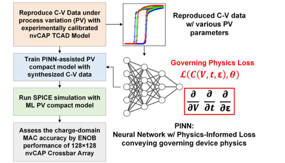
IRPS (International Reliability Physics Symposium) 2026 was my first time presenting at a conference! I presented how custom physics-informed loss functions can guide neural network compact models to stay physically consistent, here applied to process variation (PV) in ferroelectric non-volatile capacitor (nvCAP) crossbar arrays.


Motivation: Process Variation in Scaled nvCAP
The ferroelectric nvCAP is a promising device for non-destructive read and charge-domain compute-in-memory. So far, nvCAP data have mostly been measured at the µm scale, but as devices shrink to the nm regime, stochastic fabrication variations—ferroelectric thickness, dielectric constant, work function—can cause large deviations in device characteristics. Projecting yield and accuracy at future nodes requires a predictive PV-aware compact model.
Each compact modeling approach has a trade-off:
| Modeling Method | Advantages | Limitations |
|---|---|---|
| Physics-based Model (TCAD) | High physical fidelity; captures internal states | Computationally expensive; effort-intensive calibration |
| Data-driven Model (MLP) | Fast inference; simple implementation | Physical inconsistency; risk of unphysical oscillations |
| PINN Model (This work) | Physics-aware accuracy; robust generalization | Requires custom loss function design |
Neural network compact models offer > 105× inference speedup over physics-based solvers, but a pure black box can violate physical laws between training points. Our goal is to keep the speed of an MLP while forcing it to respect the physics.
Device and TCAD Data Under Process Variation
We study a 3D fin nvCAP with an ALD-grown W-doped In2O3 (IWO) oxide semiconductor layer in series with a ferroelectric Hf0.5Zr0.5O2 (HZO) layer. The capacitance is high (Con) when the IWO is accumulated and low (Coff) when it is depleted, and the ferroelectric polarization sets which state is read at Vread = 0 V.
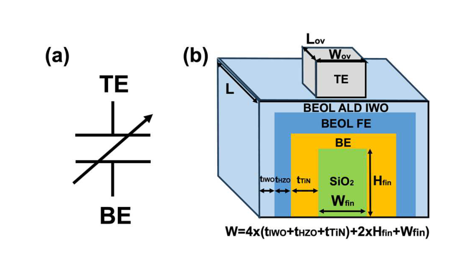
Since statistical variation data at these dimensions do not exist yet, we used an experimentally calibrated Sentaurus TCAD nvCAP model to synthesize C-V data over three process corners:
| Sweep Parameter | Default Value | Variation (3 Process Corners) |
|---|---|---|
| HZO Dielectric Constant (εHZO) | 14 | Nominal ± 10%: {12.6, 14, 15.4} |
| HZO Thickness (tHZO) | 7 nm | Nominal ± 10%: {6.3, 7, 7.7} nm |
| Bottom Electrode Work Function (WF) | 4.5 eV | Nominal ± 0.1 eV: {4.4, 4.5, 4.6} eV |
| Overlap Width (Wov) | 40 nm | {4, 10, 40} nm |
(Default design: W = 200 nm, L = 100 nm, Lov = 25 nm)
Physical Trends (What the Model Must Respect)
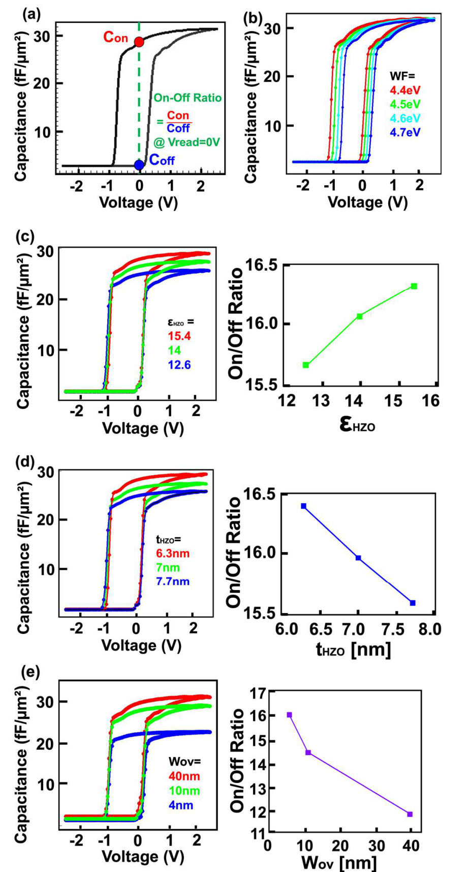
- Work function: shifts the C-V curve laterally (built-in field offset).
- εHZO ↑ / tHZO ↓: both Con and Coff increase, since capacitance is governed by CHZO ∝ εHZO/tHZO. The on/off ratio also increases, because Con depends almost entirely on CHZO while Coff is a series combination with the depletion capacitance.
- Wov ↓: absolute capacitance decreases (smaller overlap area), but the on/off ratio increases because Coff scales with the overlap area while Con is preserved by accumulation extending beyond the overlap.
These are exactly the monotone relationships that we later encode into the loss function.
Methodology: PINN with Monotonicity Constraints
Architecture
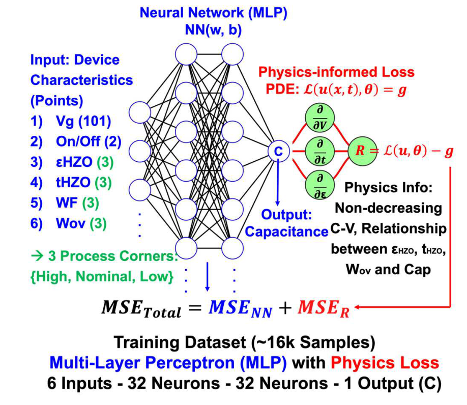
The compact model is a small 6-32-32-1 MLP:
- Inputs (6): gate voltage Vg, a binary on/off branch indicator (Con vs. Coff branch of the ferroelectric hysteresis), and four PV parameters (εHZO, tHZO, WF, Wov).
- Output (1): capacitance C.
- Training data: ~16k points from TCAD, swept over a coarse 3-corner grid (Nominal, +10%, −10%) to emulate a realistic, data-efficient design of experiments.
Why Monotonicity?
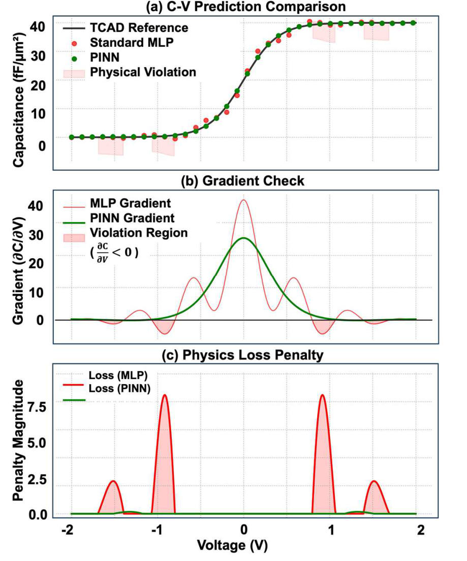
With only three corners per parameter, a standard MLP easily fits the training points but produces ripples and staircase artifacts in between. A small ripple may look harmless, but a non-monotonic C-V is physically wrong (capacitance must not decrease as Vg sweeps through the switching transition), and it can cause convergence failures in array-level SPICE simulation.
ReLU-Based Physics Loss
The total loss combines the data fit with a weighted sum of physics penalties:
The key building block is \(ReLU(x) = \max(0, x)\), which acts as a conditional filter: it is zero when the physics is satisfied and positive only when it is violated. Using automatic differentiation, we compute the partial derivatives of the predicted capacitance with respect to the inputs during training and penalize negative C-V slopes:
If \(\partial C / \partial V \geq 0\) (physically correct), the penalty is exactly zero; any negative slope produces a positive loss that the optimizer must remove. We extend the same idea to the process trends from TCAD, so that capacitance decreases with tHZO and increases with εHZO and Wov:
with \(\lambda_V = 0.05\) and \(\lambda_t = \lambda_\varepsilon = \lambda_W = 0.01\), chosen to balance the derivative magnitudes so the physics term guides the fit without overwhelming the data term. Unlike generic regularization (e.g., weight decay), these inequality constraints create a physical boundary that guides the optimizer even in regions with no training data.
Note) The same monotone-constraint idea later became the monotonicity loss for retention time in our PINO surrogate for Fe-VNAND (ICMC 2026), where trapped charge and remnant polarization must decay monotonically.
Results
1. Interpolation to an Unseen Process Corner
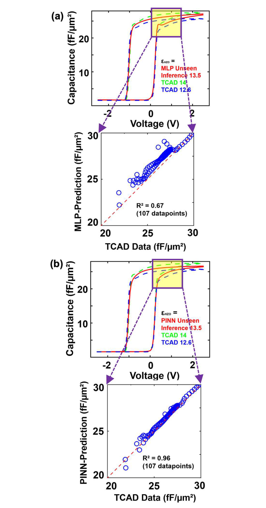
We tested both models on an unseen, experimentally calibrated εHZO = 13.5, between the trained 12.6 and 14 corners, focusing on the steep transition region (20–30 fF/µm²):
- Standard MLP: R2 = 0.67, with unphysical oscillations.
- PINN: R2 = 0.96, smooth and closely matching TCAD.
Interestingly, the standard MLP had a lower training MSE (1×10⁻⁵) than the PINN (3×10⁻⁵). The lower number reflects overfitting to the sparse grid; the slightly higher PINN training loss is the expected price of the physics constraints, and it buys robust generalization.
2. Monte Carlo Variation of Con / Coff
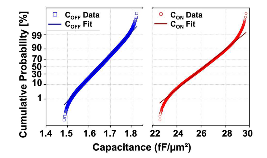
Monte Carlo sampling of the compact model (varying εHZO, tHZO, WF, with Wov = 4 nm to maximize the on/off ratio) shows Con spanning ~22–30 fF/µm² and Coff ~1.5–1.9 fF/µm². The relative variation is comparable for both states (~20–30%).
3. Array-Level Impact: 128×128 Capacitive Crossbar
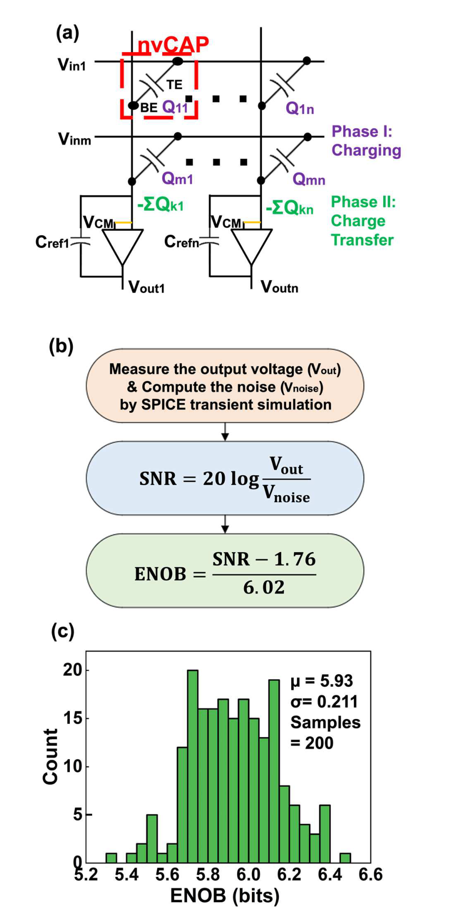
Plugging the PINN compact model into SPICE for a 128×128 nvCAP crossbar (charging + charge transfer phases), with thermal, jitter, and flicker noise, we computed the ENOB of the charge-domain MAC output. Device-level PV makes the ENOB vary from 6.49 bits down to a worst case of 5.33 bits (μ = 5.93, σ = 0.211 over 200 samples), a ~20% variation. Since low-precision neural network inference typically needs > 5–6 bits, this calls for tighter process control or PV-aware design.
Summary
- PINN Compact Model: A 6-32-32-1 MLP trained on sparse 3-corner TCAD data, with ReLU-based physics losses enforcing monotone C-V behavior and correct εHZO, tHZO, Wov scaling trends.
- Accuracy: R2 improved from 0.67 (MLP) to 0.96 (PINN) on an unseen process corner, with no unphysical ripples.
- SPICE-Ready: Monotone, smooth C-V predictions avoid convergence failures in large-array circuit simulation.
- Reliability Insight: PV causes ~20% ENOB variation in a 128×128 nvCAP crossbar, highlighting the need for PV-aware design.
Figures in this post: © 2026 IEEE. Reprinted, with permission, from G. Jeong, J. Kwak, M. Vadlamani, J. Lee, and S. Yu, “Physics-Informed Neural Network-Assisted Compact Modeling for Process Variation in Non-volatile Capacitive Crossbar Arrays,” IEEE International Reliability Physics Symposium (IRPS), 2026. IEEE Xplore
Enjoy Reading This Article?
Here are some more articles you might like to read next: